Partie 1 Extraction des données et pré-traitement

1 Extraction des données

# ------------------------------------------------------------------------------
#                   CHARGEMENT ET PRÉ-TRAITEMENT DES DONNÉES
# ------------------------------------------------------------------------------
library(rgbif)
library(dplyr)
library(sf)
library(maps)

tigre_moustique_data <- occ_search(
  scientificName = "Aedes albopictus",
  country = "FR",
  limit = 2210,
)$data

dim(tigre_moustique_data)

[1] 2210  173

head(tigre_moustique_data)

# A tibble: 6 × 173
  key        scientificName   decimalLatitude decimalLongitude issues datasetKey
  <chr>      <chr>                      <dbl>            <dbl> <chr>  <chr>     
1 6352491641 Aedes albopictu…            43.6             3.83 cdc,c… 50c9509d-…
2 6236277830 Aedes albopictu…            44.0             4.37 cdc,c… 50c9509d-…
3 6251939228 Aedes albopictu…            42.5             2.93 cdc,c… 50c9509d-…
4 6273479052 Aedes albopictu…            45.5             4.51 cdc,c… 50c9509d-…
5 6274153825 Aedes albopictu…            45.8             4.93 cdc    50c9509d-…
6 6320515685 Aedes albopictu…            43.6             3.84 cdc,c… 50c9509d-…
# ℹ 167 more variables: publishingOrgKey <chr>, X.CitizenScience. <chr>,
#   installationKey <chr>, hostingOrganizationKey <chr>,
#   publishingCountry <chr>, protocol <chr>, lastCrawled <chr>,
#   lastParsed <chr>, crawlId <int>, projectId <chr>, basisOfRecord <chr>,
#   occurrenceStatus <chr>, taxonKey <int>, kingdomKey <int>, phylumKey <int>,
#   classKey <int>, orderKey <int>, familyKey <int>, genusKey <int>,
#   speciesKey <int>, acceptedTaxonKey <int>, acceptedScientificName <chr>, …

2 RESUME DES DONNÉES

summary_table <- tigre_moustique_data %>%
  filter(!is.na(year), !is.na(stateProvince)) %>%  
  group_by(year, stateProvince) %>%                 
  summarise(n_occurrences = n(), .groups = "drop") 

nrow(summary_table)

[1] 94

library(DT)
datatable(summary_table)

3 VISUALISATIONS DES DONNEES

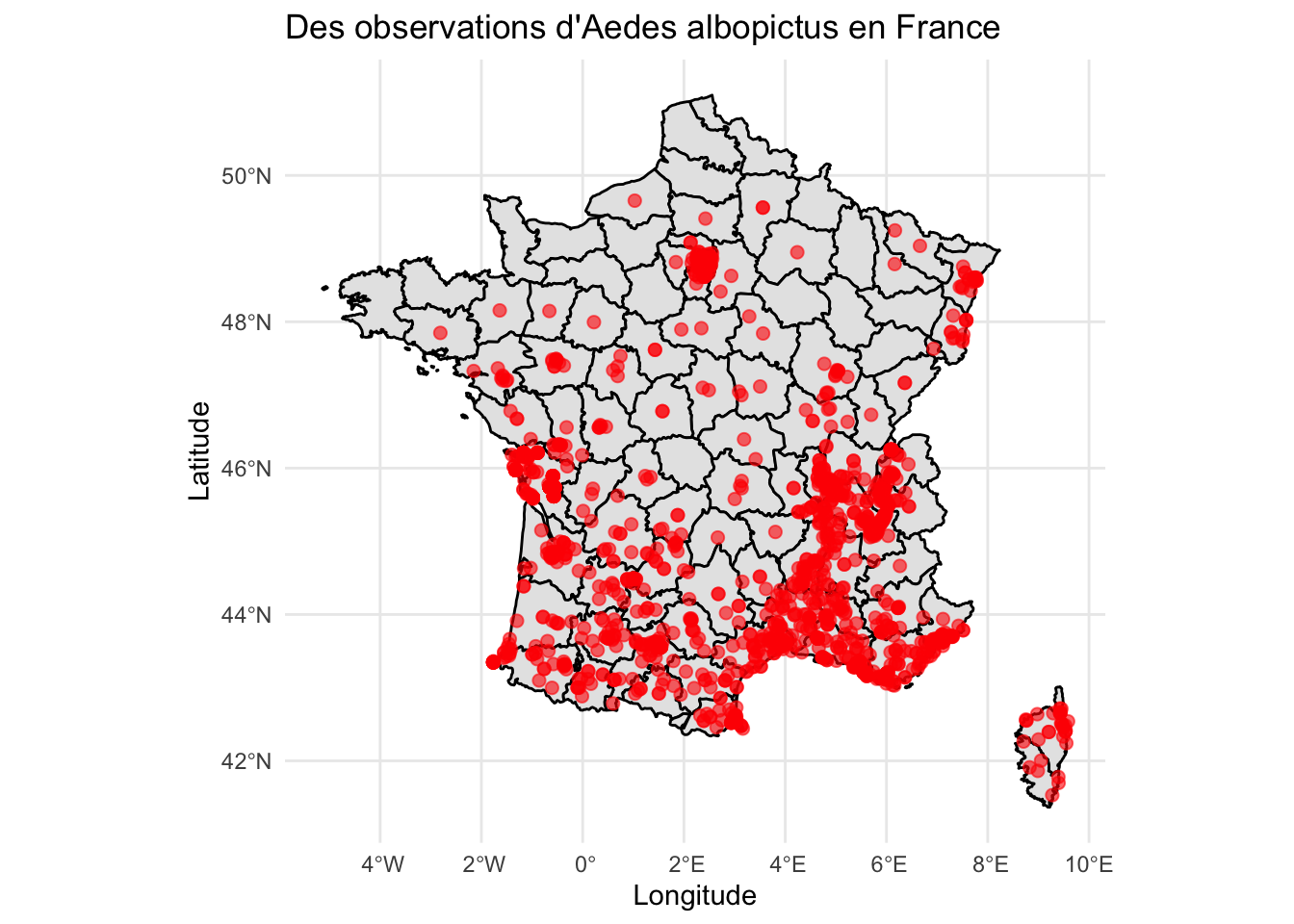
library(sf)
library(ggplot2)
library(maps)


# enlever les lignes qui n'ont pas de coordonne 

options(repr.plot.width = 20, repr.plot.height = 12)
spatial_data <- tigre_moustique_data %>%
  filter(!is.na(decimalLatitude), !is.na(decimalLongitude))
spatial_sf <- st_as_sf(
  spatial_data,
  coords = c("decimalLongitude", "decimalLatitude"),
  crs = 4326   # CRS WGS84
)

france_map <- map_data("france")

ggplot() +
  geom_polygon(
    data = france_map,
    aes(x = long, y = lat, group = group),
    fill = "gray90", color = "black"
  ) +
  geom_sf(
    data = spatial_sf,
    color = "red",
    size = 2,
    alpha = 0.6
  ) +
  theme_minimal() +
  labs(
    title = "Des observations d'Aedes albopictus en France",
    x = "Longitude",
    y = "Latitude"
  )

3.1 Par année

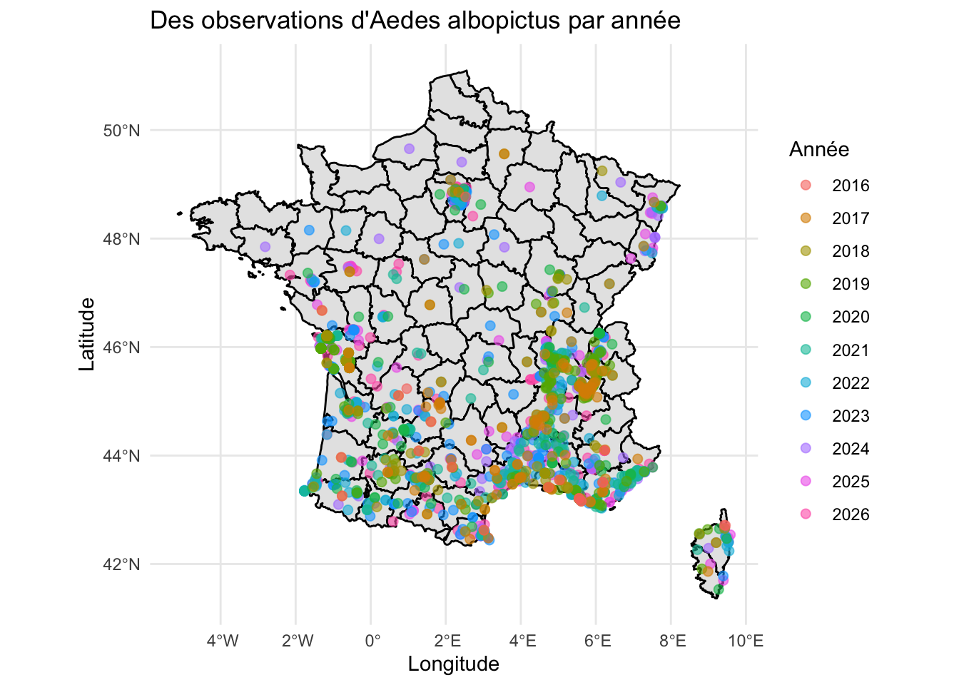
# Par année
options(repr.plot.width = 20, repr.plot.height = 12)
ggplot() +
  geom_polygon(
    data = france_map,
    aes(x = long, y = lat, group = group),
    fill = "gray90", color = "black"
  ) +
  geom_sf(
    data = spatial_sf,
    aes(color = factor(year)),
    size = 2,
    alpha = 0.6
  ) +
  theme_minimal() +
  labs(
    title = "Des observations d'Aedes albopictus par année",
    color = "Année",
    x = "Longitude",
    y = "Latitude"
  )

La carte montre une expansion progressive du moustique tigre en France entre 1999 et 2025. Initialement concentrées dans les régions du sud, les observations se sont progressivement étendues vers le nord, atteignant récemment la région parisienne et le nord-est du pays.

Cette progression s’explique en partie par l’augmentation des températures et l’évolution des conditions climatiques, qui favorisent la survie et la reproduction du moustique dans des régions auparavant moins propices à son développement.

3.2 Par site

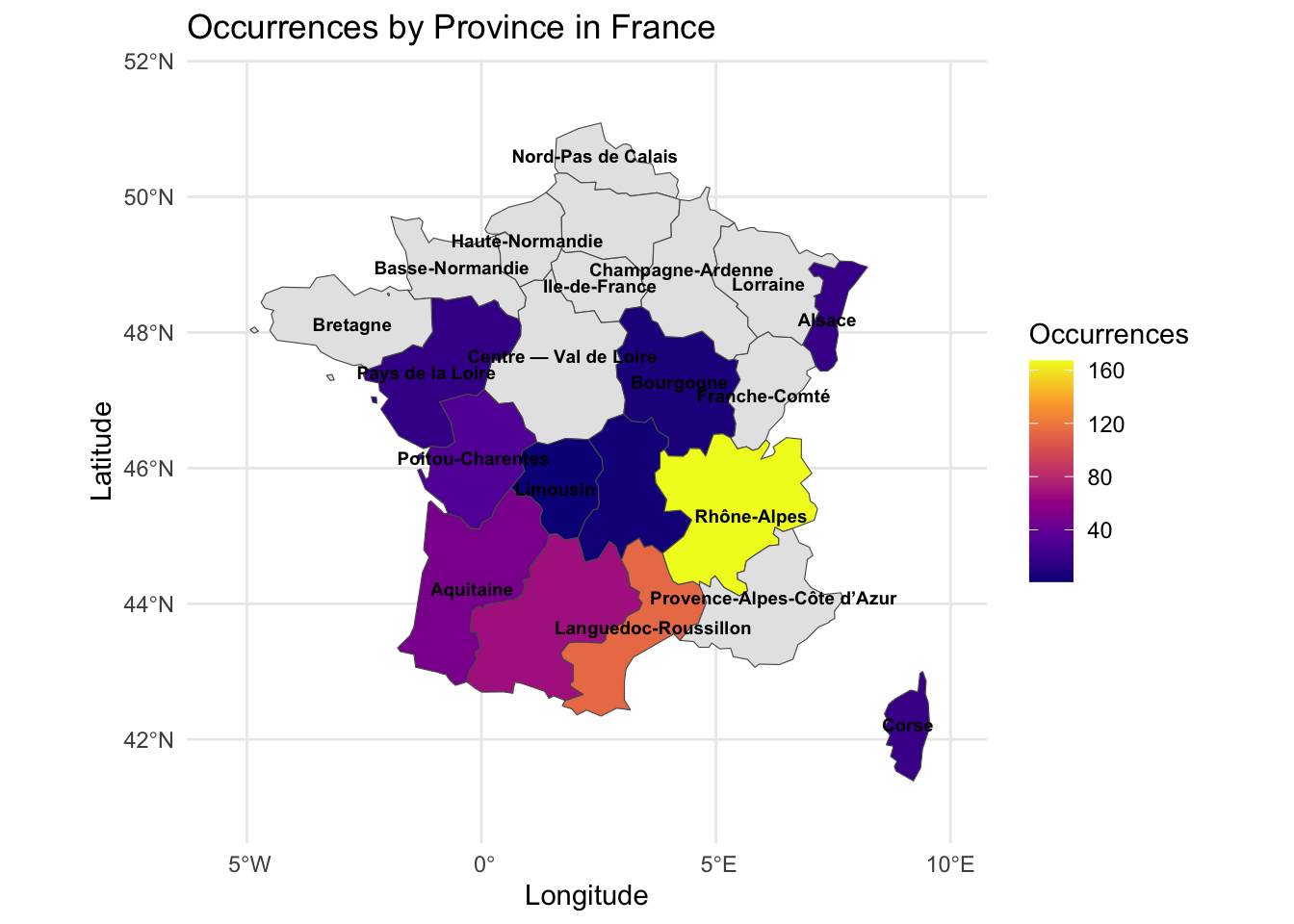
# Par site 
df <- summary_table

library(tidyverse)
library(giscoR)

options(repr.plot.width = 20, repr.plot.height = 12)
# 1.Resume les donnes
occurrence_counts <- df %>%
  group_by(stateProvince) %>%
  summarise(n = sum(n_occurrences, na.rm = TRUE))

# 2. Prend la carte
france_map <- gisco_get_nuts(country = "FR",nuts_level = 2, resolution = "20")

# 3. Ajouter les donnes
map_data <- france_map %>%
  left_join(occurrence_counts, by = c("NAME_LATN" = "stateProvince"))

# 4. Plot
ggplot(data = map_data) +
  geom_sf(aes(fill = n)) +
  geom_sf_text(aes(label = NAME_LATN),size = 2.5,color = "black",check_overlap = TRUE,fontface = "bold") +
  scale_fill_viridis_c(option = "plasma",na.value = "grey90",name = "Occurrences") +
  theme_minimal() +
  labs(title = "Occurrences by Province in France",
    x = "Longitude", y = "Latitude") +
  coord_sf(xlim = c(-5.5, 10), ylim = c(41, 51.5))

La carte met en évidence une forte concentration du moustique tigre dans le sud et le sud-est de la France. La région Rhône-Alpes apparaît comme le principal foyer, suivie par Provence-Alpes-Côte d’Azur et Languedoc-Roussillon.

Les régions de l’ouest et du centre présentent également une présence croissante du moustique, tandis que les régions du nord restent relativement peu touchées. Cette répartition reflète l’expansion progressive de l’espèce depuis les zones les plus favorables sur le plan climatique.